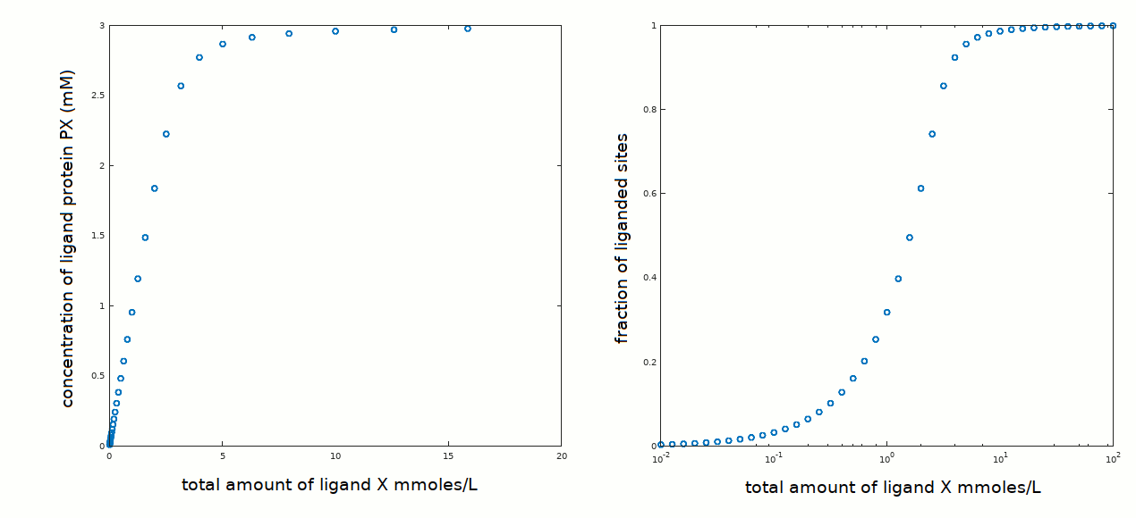
answer 5-2: qualitative analysis of the ligand binding plots
We consider first the [PX] versus [X]tot (left panel) and we observe that ligand binding is essentially a straight line up to the plateau corresponding to [PX]=[P]tot ([P]tot = 3 mM). The mid point of this line has approximate coordinates [X]tot ≅ 1.5 mM, [PX] ≅ 1.5 mM. This implies that saturation of half the available binding sites occurs when [X]free = [X]tot - [PX] ≅ 0 ! This is obviously an approximation: [X]free cannot be zero; but it is close to zero and to all effects undetectable, unless we adopt some special strategy (e.g. directly measuring [X]free using a suitable electrode, if one exists, or via labelling X with a radioactive isotope).

We now turn our attention to the fraction of liganded sites (Y) versus log [X] and we observe that the curve is strongly asymmetric, something that is not compatible with a monomeric, single ligand binding site protein.
We already observed these features in the case of a high affinity ligand (see tutorial #4), but in that case we had a non-zero estimate of [X]free at Y=0.5. We can tabulate the results we obtained in tutorials #1, #4 and #5 as follows:
| tutorial #1 | Y=0.5 at [X]free ≅ [X]tot Kd >> [P]tot |
| tutorial #4 high affinity ligand | Y=0.5 at [X]free < [X]tot 0.5 [P]tot < Kd < 5 [P]tot |
| tutorial #5 very high affinity ligand | Y=0.5 at [X]free ≅ zero; [X]tot=[PX] Kd << [P]tot |
Proceed to the next step.