Andrea Bellelli, Dipartimento di Scienze Biochimiche "A. Rossi Fanelli", Sapienza Universita' di Roma
A lecture presented at the FEBS Advanced Course "Ligand Binding: Theory and Practice" (Nove Hrady, 2-10 July 2016)
Abstract
Cooperative ligand binding is a fundamental function of a large number of proteins, whose physiological relevance spans from transport, catalysis and regulation of the cell cycle. The reversible oxygen combination to hemoglobin is a prototype of cooperativity and has been convincingly demonstrated to be a consequence of allostery, the ability of the protein to adopt either of (at least) two structural and energy states. The simplest theoretical framework that correlates cooperativity and allostery is the two-state model originally proposed by Monod, Wyman and Changeux (MWC) in 1965, whose critical assumption is that of perfect structural symmetry.
This lecture is meant to provide a general intrduction to some crucial properties of, and concepts relating to, cooperativity and allostery, namely:
1) a taxonomy of chemical linkage types
2) heterotropic linkage
3) homotropic linkage
4) cooperativity as a special case of linkage
5) homotropic and heterotropic linkage in hemoglobin
6) the two-state model of cooperativity and some of its alternatives.
1. The discoveries of homotropic and heterotropic linkage.
In 1904 Bohr, Hasselbalch and Krogh published, in the same paper, two momentous biochemical discoveries, under the title "Concerning a Biologically Important Relationship - The Influence of the Carbon Dioxide Content of Blood on its Oxygen Binding" (an english translation of the original paper may be read here). They had found that:
(i) the O2 affinity of hemoglobin (Hb) increases as the gas concentration (or partial pressure) increases. This effect was, and still is, called coooperativity. Cooperative O2 binding by Hb was the first member of a large class of events that we call homotropic linkage.
(ii) The O2 affinity of Hb decreases as the hydrogen ion and carbon dioxide concentrations increase. The effect of pH is appropriately called the Bohr effect. These phenomenona were the first instances of the large class of events that we call heterotropic linkage.
Bohr was a physiologist and the physiological relevance of his discoveries was fully clear to him; however their implications for physical chemistry were largely in advance of the time and were not fully appreciated until much later.
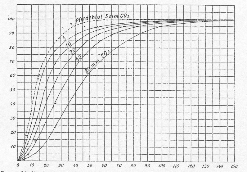
Figure 1.1: Bohr's original data on oxygen saturation of dog Hb as a function of pO2 and pCO2.
2. A general definition of chemical linkage.
Linkage occurs whenever a (biological) macromolecule binds two or more ligands to the same, or to equivalent, or to different sites; and each ligand influences the binding affinity of the other(s).
Thermodynamics dictates that if ligand #1 influences the affinity of the macromolecule for ligand #2, then the opposite is also true, and ligand #2 affects the affinity for ligand #1, in the same direction. This point (and many others) were demonstrated by Jeffries Wyman in 1948, and in an extended form, in 1964.
For the purposes of this lecture, we adopt the definitions by Wyman and Gill, i.e.:
(i) if two different ligands compete for the same binding site of the macromolecule, we have a case of identical linkage: e.g. O2 and CO competing for the heme iron of myoglobin (Mb).
(ii) if two (or more) molecules of the same ligand bind to two (or more) equivalent binding sites of the same macromolecule, we have a case of homotropic linkage: e.g. O2 and Hb,Hb being a tetramer and binding four molecules of O2. If the ligand affinity increases as more ligand is bound we have positive homotropic linkage (i.e. cooperativity); otherwise we have negative homotropic linkage.
Take home message #1: homotropic linkage requires more than one binding site for the same ligand (e.g. the protein might be an oligomer of identical or equivalent subunits like Hb, which is a tetramer made up by two alpha and two beta subunits).
(iii) if two (or more) different ligands bind to two (or more) non equivalent binding sites we have heterotropic linkage (positive if each ligand increases the affinity for the other, negative otherwise): e.g. the Bohr effect or the effect of DPG on the O2 affinity of Hb.
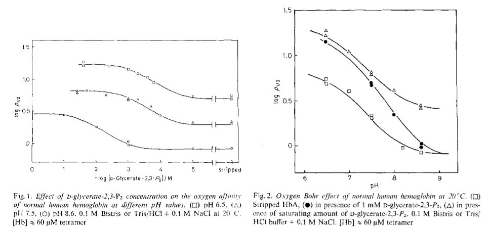
Figure 2.1: Bohr effect of and DPG binding to human Hb, as measured from the p50 of O2 by Antonini et al., 1982.
3. The physical chemistry of heterotropic linkage with 1:1 stoichiometry.
The thermodynamics of linkage was first analyzed by Jeffries Wyman in 1948.
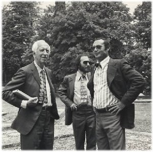
Figure 3.1: "Professor" Jeffries Wyman with Eraldo Antonini and Robert W. Noble (c. 1975).
The chemical reaction scheme for a protein (P) binding two different ligands (L and M) to two different sites is as follows:
Scheme 3.1
| KL = [P] [L] / [PL] | (eqn. 3a) |
| KM = [P] [M] / [PM] | (eqn. 3b) |
| MKL = [PM] [L] / [PML] | (eqn. 3c) |
| LKM = [PL] [M] / [PML] | (eqn. 3d) |
The energy profile in the figure is depicted for the case of negative heterotropic linkage, i.e. MKL > KL. This is evident because the energy step leading from P to PL is greater than the one from PM to PML; in the case of positive linkage the opposite would apply.
One can imagine this thermodynamic system as depicted below:
Figure 3.2
Four states of P are populated in our system: P, PM, PL, PML (the last two being represented in Fig. 3.1); we can chose any of them as the reference species and express all the concentrations as multiples of a function of the concentration of the reference species (the resulting mathematical expression is called the binding polynomial of P). We take P as the reference species and we obtain:
| [PL] = [P] [L] / KL | (eqn. 3e) |
| [PM] = [P] [M] / KM | (eqn. 3f) |
| [PML] = [PM] [L] / MKL = [P] [M] [L] / (KM MKL) | (eqn. 3g) |
| [PML] = [PL] [M] / LKM = [P] [M] [L] / (KL LKM) | (eqn. 3h) |
The last two equations yield:
KM MKL = KL LKM or LKM = KM MKL / KL (eqn. 3i)
Take home message #2: as a consequence of energy conservation, one of the equilibrium constants of a thermodynamic square can be derived from the other three.
The binding polynomial of P results:
[Ptot] = [P] (1 + [L]/KL + [M]/KM + [M][L]/KMMKL) (eqn. 3j)
It is important to keep track of the chemical meaning of the terms of the binding polynomial: the first represents [P], the second [PL], the third [PM] and the fourth [PML].
The fractional saturation of P with L results:
YL = ([PL] + [PML]) / ([P] + [PL] + [PM] + [PML]) =
= ([L]/KL + [M][L]/KMMKL) / (1 + [L]/KL + [M]/KM + [M][L]/KMMKL) =
= [L] (MKLKM + [M]KL) / [KLMKL (KM + [M]) + [L] (KMMKL + [M]KL)] (eqn. 3k)
We remark that:
(i) if MKL = KL, the presence of M has no effect on the binding of L, and our equation reduces to:
YL = [L] / (KL + [L])
(ii) if [M] = 0 (and, of course [PM] = 0 and [PML] = 0) our equation reduces to:
YL = [PL] / ([P] + [PL]) = [L] / (KL + [L])
(iii) if [M] >> KM and [M] >> LKM = KMMKL/KL (this condition implies that only protein species containing M are populated, i.e. [P] = 0 and [PL] = 0), our equation reduces to:
YL = [PML] / ([PM] + [PML]) = [L] / (MKL + [L])
If none of the above conditions apply, we should use the full equation for YL and we obtain a value of KL app which is intermediate between KL and MKL.
The experiment is usually carried out at fixed concentration of M and variable concentration of L, and one can rewrite for simplicity eqn. 3k using the following terms:
α = MKLKM + [M]KL
β = KLMKL (KM + [M])
YL = [L] α / (β + [L] α) = [L] / (β/α + [L]) (eqn. 3k')
Eqn. 3k' describes a hyperbola, and is identical to a simple binding equation, except that the apparent dissociation constant, β/α, is a complex convolution of three constants (KL, MKL, and KM) and one variable ([M], which however is kept constant during each single determination).
If several binding curves of L, each at one fixed concentration of M to cover a range of [M] that spans between [M] = 0 and [M] >> KM, are recorded, it is possible to plot the apparent equilibrium constants obtained (β/α) as a function of [M]. The following function is obtained:
β/α = KLMKL (KM + [M]) / (MKLKM + [M]KL) = MKL ([M] + KM) / ([M] + LKM) (eqn. 3l)
Take home message #3: Eqn. 3l demonstrates that the apparent dissociation constant of (PL + PML) is a hyperbolic function of [M], from which KM can be derived. Thus if binding of ligand M gives no signal or is difficult to detect, one can measure the affinity of ligand L at various concentrations of M and derive KM from the dependence of the apparent KL on [M].
Heterotropic linkage in a monomeric protein: ligand M changes the affinity of the protein for ligand L, but does not cause cooperativity. Ligand binding isotherms are hyperbolic, and simply right (or left) shifted. The L1/2 is a hyperbolic function of [M].
Warning: The demonstration given above is meant to clarify the theoretical aspects of heterotropic linkage. However clarity does not equal statistical soundness: a perfectly equivalent but statistically sounder procedure is to collect all the experimental points from all the experiments and to globally fit the values of YL to the following function of [L] and [M]:
YL = [L] / [ [L] + MKL ([M] + KM) / ([M] + LKM)] (eqn. 3m)
This is because fitting each L binding curve to a hyperbola to obtain a series of β/α, and this series to a second hyperbola distorts the distribution of the experimental errors.
4. Linkage is key to life.
Because of linkage, biological macromolecules "sense" their environment and "adapt" or "respond" to it, two fundamental functions of organisms. E.g. Hb senses the acidity of the medium and responds to it by releasing the bound O2; receptors sense the presence of their effectors and respond by transmitting a signal; and so on. J. Wyman called these features the "cybernetics of macromolecules".
5. A short detour: Ligand binding to the non cooperative symmetric oligomer.
We now consider the case of a homodimeric protein, made up of two identical subunits that do not undergo structural changes upon ligation. Many proteins having enzymatic or carrier functions are symmetric oligomers made up of identical or nearly identical subunits: e.g. this is the case of Hbs, Hcys, Trx reductase, amine oxidases, etc. The thermodynamic properties of the oligomer will be described for the simplest possible case, that of a symmetric homodimer:
P + 2 L <==> PL + L <==> PL2 (eqn. 5a)
In this system each subunit binds one molecule of the ligand and is insensitive to what happens to its partner in the dimer, hence the binding polynomial and the fractional saturation for the subunits are identical to the ones we wrote for the monomeric protein. However, we may not be satisfied with the above description, and we may ask how liganded and unliganded subunits are distributed within dimers, i.e. to what extent singly and fully liganded dimers are populated. In the absence of favorable or unfavorable interactions between monomers in the dimer, the distribution of liganded and unliganded subunits within dimers is expected to be statistical, i.e. binomial:
[fraction of unliganded subunits + fraction of liganded subunits]number of binding sites = [ (K / K+[L]) + ([L] / K+[L]) ]2 (eqn. 5b)
It is important to keep track of the chemical meaning of each term: the exponent represents the number of subunits in the protein, the first term the fraction of unliganded subunits, the second the fraction of liganded subunits, and their sum equals one. When we develop the expression, we obtain:
( K2 + 2 K [L] + [L]2 ) / (K + [L])2 (eqn. 5c)
which again equals one and whose three terms represent the fractions of unliganded, singly and doubly liganded dimers respectively. If we equate [P] = [P]tot K2 / (K + [L])2 , and divide the terms of (eqn. 5c) by [P], we obtain the binding polynomial:
[P]tot = [P] (1 + 2 [L]/K + [L]2/K2) (eqn. 5d)
If we now write down the equation of the fractional saturation for the dimer, taking into account that the number of liganded sites is one for the singly liganded dimer and two for the doubly liganded, and that the total number of sites per molecule is 2, we obtain:
Y = (2 K[L] + 2 [L]2) / 2 (K + [L])2 = [L]/K (1 + [L]/K) / (1 + [L]/K)2 (eqn. 5e)
From the binding polynomial ((eqn. 5d)), we may derive the apparent dissociation constants for the singly and doubly liganded dimers:
| dissociation constant of the diliganded dimer: | K2, app = [PL] [L] / [PL2] = 2 K | (eqn. 5f) |
| dissociation constant of the monoliganded dimer: | K1, app = [P] [L] / [PL] = K / 2 | (eqn. 5g) |
The binding polynomial for the homodimer we obtain from the apparent dissociation constants is identical to the one we obtain from the binomial distribution of liganded and unliganded subunits:
[P]tot = [P] (1 + [L]/K1, app + [L]2/K1, appK2, app) = [P] (1 + 2 [L]/K + [L]2/K2) (eqn. 5h)
Obviously, in this case the value of Y is the same one would obtain ignoring the distribution od the subunits in the dimers and simply applying the equation for a single site: Y = [L] / (K + [L]). If, however, symmetry were to be broken for any reason, so that the intrinsic ligand affinity of the two sites were different, and eqns. 5f and 5e were to be replaced by mnore complex functions (always maintaining the statistical factors), one would obtain:
YL = ([L]/K1, app + 2[L]2/K1, appK2, app) / 2 (1 + [L]/K1, app + [L]2/K1, appK2, app) (eqn. 5i)
An explanation of the statistical coefficients of the homodimer (or, in general terms of the oligomer) is that when we try to write down the binding polynomial for the homodimer, we should take into account that each macromolecule contains two "first" binding sites and only one "second" binding site: i.e. there is a statistical bias for a ligand to dissociate from a doubly liganded dimer rather than from a monoliganded one. We thus have two apparent equilibrium constants, one for the dissociation of the diliganded homodimer and one for the monoliganded homodimer, even though the "intrinsic" ligand affinity of each site is the same, irrespective from the fact that it occurs in a singly- or doubly-liganded homodimer.
Take home message #4: the relative population of ligation intermediates of a protein oligomer depends on the intrinsic binding constants and the pertinent statistical factors.
6. In a symmetric oligomer heterotropic linkage may be a cause of cooperativity.
What happens if we have heterotropic linkage in a homodimer? We shall consider only the simplest case, i.e. the thermodynamically symmetric homodimer, whose monomers are equivalent and non cooperative for the first ligand both in the presence and in the absence of the second ligand:
Scheme 6.1
Because of the symmetry postulates we applied, the equilibrium constants are the same as in the case of the monomer, considered above (eqns. 3a to 3d), with the only addition of LLKM. The reason why we need this additional constant is that the system composed by the L- monoliganded and diliganded species forms a second thermodynamic square, analogous to the one described by (eqn. 3i):
LKM MKL = KL LLKM or LLKM = LKM MKL / KL = KM (MKL / KL)2 (eqn. 6a)
We also remark that the energy profile is again depicted for the case of negative heterotropic linkage, and that depending of the concentrations of [M] and [L], the preferred species would be those highlighted in red, with the order of appearance indicated by the arrows. Thus, if we start with the protein and nothing else in solution we only have P; when we add M, PM becomes populated; and as we increase the concentration of L we populate first PML and next PL2, while M is released. The dashed circle indicates the area of the energy profile which corresponds to the one considered in the above paragraph 4.
A graphical representation of our system, which highlights the symmetry of the two binding sites is as follows:
Figure 6.1
We can now write down the binding polynomial for the system described in Fig. 6.1, and as always we take unliganded P as the reference species (remember that we need to take into account the statistical factors!):
| [PL] = [P] 2[L]/KL | (eqn. 6b) |
| [PL2 ] = [P] [L]2 / KL2 | (eqn. 6c) |
| [PM] = [P] [M]/KM | (eqn. 6d) |
| [PML] = [P][M] 2[L]/KM MKL | (eqn. 6e) |
| [PML2 ] = [P][M][L]2/KM MKL2 | (eqn. 6f) |
The resulting binding polynomial is:
[Ptot] = [P] (1 + 2[L]/KL + [L]2/KL2 + [M]/KM + [M]/KM2[L]/MKL + [M]/KM[L]2/MKL2) =
= [P] [(1 + [L]/KL)2 + [M]/KM (1 + [L]/MKL)2] eqn. 6.g)
From the binding polynomial one derives the fractional saturation for ligand L:
| [L]/KL (1 + [L]/KL) + [M]/KM [L]/MKL (1 + [L]/MKL) | |
| YL = | ---------------------------------------------------------------------------------- (eqn. 6h) |
| (1 + [L]/KL)2 + [M]/KM (1 + [L]/MKL)2 |
The above equation may appear difficult to apply to any practical use, except fitting a set of equilibrium dissociation isotherms of PL recorded at several values of [M] for the three parameters. However one may derive from it an apparent affinity of the protein for the ligand L at any fixed concentration of the effector M. Let us use as the apparent affinity the ligand concentration required to achieve YL = 0.5 that we call L50. It is easy to demonstrate that:
L502 = KL2 MKL2 ([M] + KM) / (KM MKL2 + [M] KL2) (eqn. 6.i)
We remark that:
i) in the absence of M, L50 = KL
ii) if [M] is saturating (i.e. high enough to saturate P irrespective of [L]), L50 = MKL
iii) under all experimental conditions different from i and ii, the square of L50 is a function of [M]; and in general, for a n-subunits oligomer, the nth power of L50 is a function of [M]. This leads to our
take home message #5: the maximum slope of the plot log (L50) vs. log (M) equals the ratio of the binding stoichiometries L:M
Under appropriate experimental conditions, eqn. 6.h, above, yields a sigmoid, i.e. cooperative, binding isotherm. One may ask how the negative heterotropic ligand M can introduce positive homotropic cooperativity for ligand L in the protein; but this question is ill conceived: as I demonstrate below, cooperativity is the consequence of symmetry, not of the binding of M. M only makes the relationship between symmetry and cooperativity evident.

Take home message #6: heterotropic linkage may induce cooperativity in an otherwise non cooperative oligomeric protein, if the symmetry requirement is fulfilled.
7. Do we really need the heterotropic effector? The two-state allosteric model by Monod, Wyman and Changeux.
In 1963 J. Monod coined the concept of allostery (greek: other structure) to describe a protein that can adopt two different three dimensional structures. Monod's interest at the time was focussed on the heterotropic regulation of enzymes; but shortly afterward he was to discover another case of allosteric regulation, namely the repressor protein of the operon Lac (for which he was awarded the Nobel Prize for Medicine and Physiology). If Wyman's interpretation of heterotropic linkage was based on a pure, disembodied thermodynamic formalism, Monod's one had a sort of esthetical connection to the shape of proteins, as real objects. Figures 3.2 and 6.1 very crudely reflect what must have been Monod's ideas. Monod was fascinated by what he called "nature's elegance" and he is reported to have said that elegance did not prove a model true, but lack of elegance demonstrated a model false.
Lack of structural symmetry in a homodimer is obviously non-elegant, and is hard indeed quite difficult to imagine, unless the monomer-monomer interface resides in a region of the protein whose structure is not affected by any ligand:

Figure 7.1: The isologous homodimer does not tolerate asymmetry.
Allostery in a protein oligomer yields a thermodynamic system similar to the one considered under the heading #6, with one important difference: the two structural states are to be considered as conformational isomers of the protein, that freely equilibrate in the absence of any ligand. The reaction pathway and energy profile of ligand binding to an allosteric homodimer is as follows:
Figure 7.2: The two-state allosteric model for a symmetric homodimer.
Given the complementarity of their views, the meeting between Wyman and Monod in Paris was bound to be especially fruitful and indeed in 1965 Jacques Monod, Jeffries Wyman and Jean Pierre Changeux co-autored a famous paper describing cooperativity as a consequence of allostery (quoted over 6800 times in the literature!). The paper itself makes an extremely stimulating reading. It starts with the premises of the allosteric model, were it is stated with outmost clarity "Allosteric proteins are oligomers, the protomers of which are associated in such a way that they all occupy equivalent positions. This implies that the molecule possesses at least one axis of symmetry". Allosteric protein, in Monod's view may undergo conformational transitions, but always retain their symmetry. The equations follow and develop the consequences of molecular symmetry. Then the principles of structural symmetry are explained in detail. Proteins are necessarily asymmetric and can form asymmetric aggregates of identical polypeptide chains via heterologous interfaces. A heterologous interface is one that involves different surface areas for the two contacting monomers, e.g. as it happens in tubulin and actin. Alternatively, two identical monomers can form a symmetric homodimer via an isologous interface. The homodimer presenting an isologous interface has 180 degrees rotational symmetry and the contact areas of the two monomers involve the same surfaces; thus each contact is present twice in the isologous interface.
Hemoglobin is a tetramer formed by two couples of polypeptide chains named α and β. The three dimensional structure of the subunits α and α is very similar, both sharing the "globin fold", made up of 8 α-helices named A through H. The interfaces are pseudo-isologous: i.e. they always involve the same structural features on an α and a β subunit (minor truly isologous contacts exist between the two α subunits whereas the two β subunits form a isologous but "loosely packed" interface). The interfaces are of two types, named α1β1 and α1β2. The contacts at the α1β1 interfaces involve helices α1B-β1H; α1G-β1G; and α1H-β1B. The contacts at the α1β2 interfaces involve the α1C helix-β2FG corner and α1FG corner-β2C-helix.
Figure 7.2: Interface contacts in the hemoglobin tetramer. Note that the C-FG distance is greater in RHb than in THb.
Strictly speaking, the intersubunit interfaces of Hb are pseudo-isologous because the contacting subunits are not identical. However a higher degree of symmetry is present since the tetramer may be imagined as made up of two identical αβ dimers. The sum of the α1β1 and α2β2 intersubunit interfaces presents a symmetry axis, all contacts occur twice and forms a unit that we called an extended isologous interface (i.e. an interface which is isologous with respect to a lower order oligomer, in this case a dimer, instead of a monomer). The same applies to the sum of the α1β2 and α2β1 interfaces. E.g. in the extended isologous interface between the α1β1 and α2β2 dimers, the contact between the α1C helix and the β2FG corner is exactly duplicated by that at α2C helix-β1FG corner.
Take home message #7: if a protein is a symmetric homooligomer of identical subunits, cooperativity (homotropic linkage of binding sites) is to be expected as an almost necessary consequence of symmetry.
What has all this to do with cooperativity? The essential point is as follows: the FG corner is contiguous to the F helix, whose eight residue is the proximal His, that coordinates the heme iron. Upon oxygen binding, the iron and the proximal His move slightly, and this movement extends to the FG corner, hence to the α1β2 interface (see Fig. 7.1). A survey by Maurizio Brunori and myself showed that the distance between the C helix and FG corner of the same subunit, be it α or β increases by approx. 1 A on oxygenation:
Due to the interface symmetry, it is impossible for one subunit to be liganded and have the C-FG distance characteristic of liganded Hb and the adjacent one to be unliganded and to have the C-FG distance characteristic of unliganded Hb (see Figures 7.1 and 7.2). Thus either the unliganded subunit assumes the structural configuration of the unliganded one or vice-versa.
Take home message #8: structural symmetry in an oligomeric protein is a type of positive homotropic linkage. This is because the ligand which binds to its site "adapts" its geometry in order to optimize affinity (i.e. to increase the free energy of binding) and, in the presence of symmetry, it also adapts in the same way the other binding sites of the oligomer. Thus: symmetry = cooperativity.
8. Alternatives to the two-state model.
The crucial postulate of the two-state model is that the cooperative protein is a symmetric oligomer stable in two different structural conformations, which equilibrate freely, even in the absence of the ligand. This postulate clearly applies to Hb, in which the structure of three of the four "extreme" conformers have been solved by X-ray crystallography (i.e. THb; THb(O2)4; RHb(O2)4). It is possible to hypothesize models of cooperativity that do not require the protein to be stable in two structural conformations (i.e. models not involving allostery). The very first model of this type was proposed by L. Pauling in 1936, and several variants were proposed thereafter. The typical feature of "sequential" models of cooperativity is that a structural change of the "induced fit" type is induced by the ligand in the liganded subunit, and is sensed by the neighbouring subunits, whose ligand affinity is affected. A modern version of sequential models is based on the common observation that ligation reduces the conformational enthropy of the polypeptide chain. The effect of enthropy reduction is schematically illustrated in fig. 8.1 for the case of the symmetric homodimer. In the absence of any ligand the protein has greater flexibility than in the presence of bound ligand; via the interface, the reduced flexibility of the bound subunit is communicated to the ligand-free subunit. Reduction of conformational enthropy upon binding lowers the ligand affinity of the first site, but not that of the second site, hence cooperativity. Notice that this is not a two-state model in that only one energy state is accessible to the protein for any given ligation state.
Figure 8.1: Schematic representation of a sequential model based on enthropy reduction.
Selected references
Angelucci et al. One ring to bind them all (on the concept of extended isologous interfaces)
Antonini et al. 1982 (on the heterotropic effects in Hb)
Baldwin and Chothia (on the structure of Hb and the allosteric structural change)
Bellelli and Brunori BBA (on the mechanism of Hb cooperativity)
Bohr Hasselbalch and Krog (the discovery of homotropica and heterotropic effects)
Monod Wyman and Changeux (the allosteric model; the original definition of the isologous interfaces)
Wyman 1948 (on chemical linkage)
Wyman 1964 (on chemical linkage)